Note, 29 September 2026: The R values in this study come from our older backtest chain. On a random market without direction that chain still books positive R, so the absolute levels here are too high, and comparisons within the chain are not proven either. Why, and what we changed: The random market as a ruler.
Re-run, 5 October 2026: The 25 combinations of breakout rule and market from our rulebook have been re-measured on the corrected chain and on real broker ticks. None has an advantage over the random market; after costs the mean is −0.08 R per trade. Positive R levels and comparisons in this study are therefore not proven. All numbers: Our own breakout rules, re-measured.
Data basis: Two populations. (A) Breakout data collection: every 5-, 10- and 15-minute candle of the session as reference candle, both break directions, stop at the opposite candle end, blunt exit without trailing; gold/FX (XAUUSD, EURUSD, GBPUSD, 4.04 million breaks) and indices (DAX, FTSE, NQ, Dow, SPX, 3.56 million breaks); effects as difference to the mean of the same market and timeframe. (B) Our episode basis: 103,182 momentum trades (fade setups excluded) or 123,193 trades including fades, 10 markets, 2015–2026, real exit mechanics (trailing stop BE 0.5 / TS 1.0 / step 0.5, or hold for the runner setups), net of spread and slippage. In-sample/out-of-sample split 2022. Candle shape and close position are known before the break — no lookahead. No trading recommendation.
Price-action literature lives on candle shapes. The hammer signals rejection, the doji indecision, the big body conviction. The question we asked is not whether these shapes exist — they do — but whether they say anything about the breakout from the candle that is not already contained in a single number: where did the candle close, relative to the side that later breaks?
That is not an academic distinction. Body ratio and close position are strongly correlated; a candle with a big body almost inevitably closes near an extreme. Measuring shape raw means measuring the close a second time. The test has to separate the two.
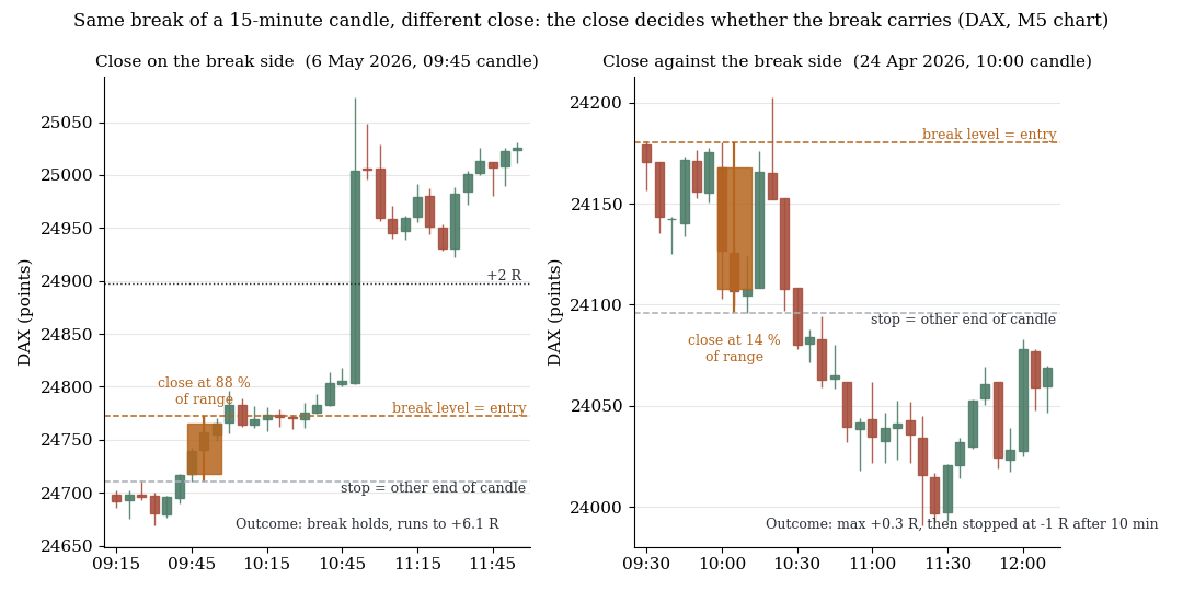
Two breaks of the same kind, DAX on 5-minute bars: on the left the reference candle closes on the break side and the break carries, on the right it closes against it and the break dies after ten minutes.
1. Shape relative to break direction (gold/FX)
Shape is read relative to the break direction: "close at the upper edge" means something different for a long break than for a short break. The metric close position is 1.0 when the candle closes exactly on the side that later breaks and 0.0 on the opposite side. Classes are disjoint, effect as difference to the market-timeframe mean.
| Class | Definition | Δ avgR | t |
|---|---|---|---|
| Close on the break side | close position ≥ 0.75 | +0.091 | +35.9 |
| Hammer | wick against the break side ≥ 0.45, body < 0.40 | +0.061 | +13.3 |
| Doji | body < 0.20 | −0.013 | −4.6 |
| Thruster | wick in break direction ≥ 0.45, body < 0.40 | −0.068 | −14.9 |
| Close against the break side | close position ≤ 0.25 | −0.100 | −38.0 |
In quintiles of close position the effect is perfectly monotonic: −0.113 → −0.057 → +0.005 → +0.064 → +0.102. Body ratio, by contrast, is almost irrelevant (−0.014 to +0.013 across classes). All three markets show the same picture.
What survives of the shape doctrine is a single contrast: hammer versus thruster, both with an equally small body, a 0.13 R spread. The wick against the break side is good, the wick in break direction is bad. Looked at closely, that too is a statement about the close: a long opposing wick with a small body means the candle closes near the break side.
For the indices the shape evaluation in this collection was not available at measurement time; the index confirmation comes from the second population.
2. Body versus close on the episode basis
103,182 momentum trades, real exits. Correlation body ratio ↔ close position: +0.25; correlation body ratio ↔ |close position − 0.5|: +0.52 — that is the actual kinship. First the raw body ratio, in quintiles:
| Body quintile | avg body | avgR | t | IS | OOS |
|---|---|---|---|---|---|
| Q1 (doji-like) | 0.10 | +0.066 | +5.0 | +0.058 | +0.079 |
| Q2 | 0.29 | +0.061 | +4.7 | +0.044 | +0.086 |
| Q3 | 0.47 | +0.043 | +3.6 | +0.016 | +0.085 |
| Q4 | 0.64 | +0.069 | +5.8 | +0.044 | +0.106 |
| Q5 (massive) | 0.84 | +0.057 | +5.1 | +0.046 | +0.072 |
Flat. No gradient, no ordering, IS and OOS without a common direction. Now the same body ratio within the close-position classes:
| Close position | body < 0.20 | 0.20–0.45 | 0.45–0.70 | > 0.70 | spread | t |
|---|---|---|---|---|---|---|
| < 25% | −0.070 | −0.156 | −0.161 | −0.131 | −0.061 | −1.1 |
| > 75% | +0.157 | +0.115 | +0.118 | +0.098 | −0.059 | −2.1 |
Within the top class the small body is even slightly better than the massive one (spread −0.059, t = −2.1) — the opposite of the body doctrine, and barely at the threshold. The doji, taken in isolation (n = 20,438, 19.8% of trades), sits at +0.067 R and decomposes entirely along the close: doji with close position > 75% +0.157 (t = +6.0; IS +0.140 / OOS +0.184), doji with close position < 25% −0.069 (t = −1.4). "Doji" is not a class. Where it closes is the class.
3. What the close actually separates — and what it does not
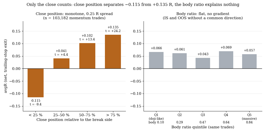
Close position separates −0.115 R from +0.135 R and is monotone; the body ratio on the same trades is flat.
| Close position | n | avgR | t | IS | OOS | avg MFE | ≥ 3 R | hit rate |
|---|---|---|---|---|---|---|---|---|
| < 25% | 12,453 | −0.115 | −9.4 | −0.121 | −0.105 | 3.56 | 42.3% | 29.0% |
| 25–50% | 18,440 | +0.041 | +4.4 | +0.033 | +0.053 | 3.57 | 42.5% | 34.5% |
| 50–75% | 26,529 | +0.102 | +13.4 | +0.076 | +0.144 | 3.38 | 40.2% | 36.7% |
| > 75% | 45,760 | +0.135 | +24.2 | +0.117 | +0.162 | 3.05 | 36.6% | 38.3% |
The spread between the weakest and strongest class is 0.25 R and stable in both periods. But the MFE columns (maximum favourable excursion, independent of the exit) contain the actual mechanism: strong breaks do not run further — they win more often. The share ≥ 3 R falls from 42.3% in the weakest to 36.6% in the strongest class, while the hit rate rises from 29.0 to 38.3%. The close says something about the probability that the break holds at all, not about the length of the run.
The consequence for the exit: the tight trailing stop is the best variant in each of the four classes (> 75%: tight +0.135, wide +0.106, very wide +0.098, hold +0.108). A wider trail for strong candles, as intuition suggests, costs 685 → 574 R per year across all classes.
4. Filters raise avgR, not automatically the yield
The obvious conclusion — drop breaks against the close side — works as a quality filter and is at the same time a warning about the metric. Pooled across all setups (first break per setup and day, n = 85,343):
| Variant | n | share | avgR | sum per day | IS | OOS |
|---|---|---|---|---|---|---|
| All first breaks | 85,343 | 100% | +0.074 | +0.074 | +0.055 | +0.102 |
| Only breaks towards the close side (≥ 0.50) | 59,902 | 70.2% | +0.112 | +0.078 | +0.089 | +0.147 |
| Only clear candles (≥ 0.75) | 38,200 | 44.8% | +0.126 | +0.056 | +0.108 | +0.153 |
| Only breaks against the close side | 25,441 | 29.8% | −0.016 | −0.005 | −0.023 | −0.006 |
avgR rises with the threshold, yield per day does not: the clear-candle variant has the highest avgR and the lowest yield. On the full basis (123,193 trades) the threshold series shows the same — R per year 628 (all) → 723 (≥ 0.50) → 672 → 587 → 525 → 442 (≥ 0.80), at avgR 0.061 → 0.104 → 0.119. And out-of-sample the yield gain of the 0.50 threshold shrinks to zero: 932 R/year against 932 without filter. The filter makes the book more efficient OOS (fewer trades, same sum), not more profitable.
Two of our setups that already select via a compression filter react the opposite way as well: there the break against the close side is the better one. Close position is not a universal filter but a feature that interacts with the setup mechanism.
5. Weekday: looks significant, does not hold
From the same breakout collection, effect as difference to the market-timeframe mean, n per weekday 687,000 to 734,000 (indices):
| Weekday | Δ avgR | t | IS | OOS |
|---|---|---|---|---|
| Monday | −0.012 | −4.3 | −0.036 | +0.025 |
| Tuesday | −0.012 | −4.4 | −0.031 | +0.018 |
| Wednesday | −0.002 | −0.5 | −0.030 | +0.043 |
| Thursday | +0.032 | +10.5 | −0.048 | +0.161 |
| Friday | −0.006 | −2.2 | −0.072 | +0.098 |
Thursday with t = +10.5 looks like a finding. The IS/OOS columns show what it is: all five weekdays are negative in-sample and positive out-of-sample. That is a period effect — breakout returns are higher from 2022 on — which a weekday effect only rides on if the period happens to fall unevenly across days. Gold/FX contradicts the indices on top (there Tuesday +0.030 and Friday +0.038 lead, Wednesday −0.036), and the per-market table is inconsistent (Dow Thursday +0.061, DAX Thursday ±0.000). An effect that switches days between asset classes and depends on the period within a class does not belong in a rulebook.
6. What this means
Candle patterns are proxies for a number. Hammer, doji, body — everything we could measure collapses onto the position of the close relative to the break side. That number is known before the break, monotonic and stable across both periods; the shapes beyond it carry nothing that survives |t| ≥ 2 and has a direction of its own at the same time.
The close is a probability feature, not a run-length feature. Strong candles raise the hit rate and shorten the tail. Deriving a wider stop from them costs money.
avgR is the wrong decision metric for filters. Every filter raises it. The question is the sum per day, and for the universal filter it is unchanged OOS. That is the same lesson as in our edge persistence study: what looks like a finding has to survive the period — the weekday did not.
7. Limits
- Two populations with different exit mechanics. The breakout collection (sections 1 and 5) uses a blunt exit without trailing and is not comparable in level to the episode figures (sections 2 to 4); only the structure within each table counts.
- Shape evaluation gold/FX only. The index shape classes were missing at measurement time; the index statement rests on body ratio and close position from the episode basis.
- Thresholds in section 4 are chosen in-sample; the OOS column is the control. We deliberately did not publish the best threshold per setup — it is in-sample selection.
- Weekday without calendar control. The event calendar (FOMC, NFP, CPI) was not available; weekday and events are not independent.
- The setup family is ours. Absolute avgR levels are optimistic; the differences between classes are the result.
📄 Full study as PDF: 8 pages incl. all tables, figures and limits (in German).
Disclaimer: Historical statistics are no guarantee of future market behaviour. This study is not investment advice. Trading involves risk of loss up to total loss.