Note, 21 October 2026: The verdict of this study used to read “edge confirmed”. It has no untouched holdout, and its R values come from the older calculation chain (see the notes below). It therefore now reads “measured”. How we test today: our workflow since October 2026.
Note, 29 September 2026: The R values in this study come from our older backtest chain. On a random market without direction that chain still books positive R, so the absolute levels here are too high, and comparisons within the chain are not proven either. Why, and what we changed: The random market as a ruler.
Re-run, 5 October 2026: The 25 combinations of breakout rule and market from our rulebook have been re-measured on the corrected chain and on real broker ticks. None has an advantage over the random market; after costs the mean is −0.08 R per trade. Positive R levels and comparisons in this study are therefore not proven. This study's statement about a persistent structural edge presupposes that the edge exists. That is not proven. All numbers: Our own breakout rules, re-measured.
Data basis: 123,193 episodes, 10 markets (DAX, FTSE, DOW, NQ, SPX, HK50, JPN225, XAUUSD, EURUSD, GBPUSD), 23 setups, 05 Jan 2015 – 05 Jun 2026 (11.4 years, 23 half-years). Exit: trailing stop BE 0.5 / TS 1.0 / step 0.5, net of spread and slippage. Unit: R (risk multiple). No trading recommendation.
Every trader has run into this. A setup that ran beautifully for six months stops working. A market that was dead wakes up. The question underneath is always the same: when I measure an edge, what does that tell me about the future — and does it tell me anything at all?
Most answers are anecdotes. This is a measurement. It asks whether the past is a forecast, and the answer turns out to be yes — but for a different part of the data than the one most people are watching.
1. The model: three things hide inside one number
If a cell — one setup, in one market, in one direction — returns +0.30 R in a half-year, that number contains four things at once:
measured = structural edge + market regime + fresh anomaly + sampling noise
- Structural edge (α): what this cell is worth permanently. Constant over time.
- Market regime (τ): the common tide that lifts or sinks every cell in that period.
- Fresh anomaly (ε): this cell behaving differently in this specific period than it usually does. This is what people mean by "the setup is running hot right now."
- Sampling noise: pure chance from a finite number of trades.
These four are not separable by eye, but they are separable arithmetically — via two-way demeaning across 85 cells × 23 half-years. And they behave completely differently. That difference is the entire point of this study.
2. How much of a measured edge is even real?
Observed variance always contains sampling noise. But the size of that noise is known — each cell-period has its own standard error. Subtract the average squared standard error from the observed variance and what remains is the real signal.
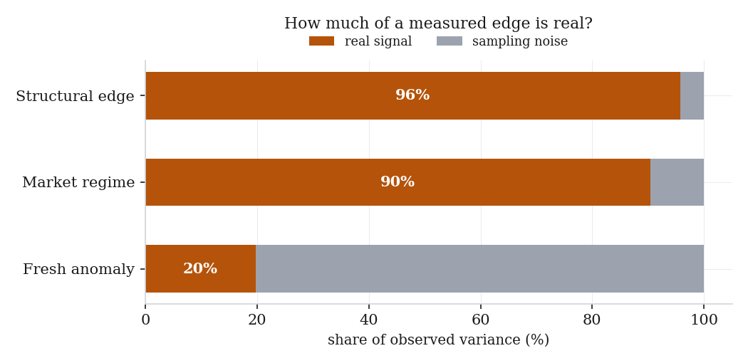
| Component | SD observed | SD noise | SD real | Real signal |
|---|---|---|---|---|
| Structural edge | 0.162 | 0.033 | 0.159 | 96% |
| Market regime | 0.055 | 0.017 | 0.052 | 90% |
| Fresh anomaly | 0.174 | 0.156 | 0.077 | 20% |
Read the last row carefully. When a cell deviates from its own norm in a given half-year, 80% of that deviation is noise. The differences between setups are almost entirely real. The differences between periods within the same setup are almost entirely not.
Note that the observed spread is nearly identical in rows one and three (0.162 vs 0.174). On the screen, a structural edge and a fresh anomaly look exactly the same size. Only the decomposition tells them apart.
3. The anomaly does not decay — it falls off a cliff
Take every cell that becomes conspicuous in a period (|t| ≥ 2 against its own norm) and follow it forward.
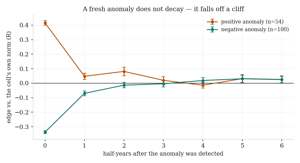
| Half-years later | 0 | 1 | 2 | 3 | 4 | 5 | 6 |
|---|---|---|---|---|---|---|---|
| after positive anomaly (n=54) | +0.416 | +0.048 | +0.081 | +0.020 | −0.014 | +0.031 | +0.026 |
| after negative anomaly (n=100) | −0.337 | −0.070 | −0.014 | −0.004 | +0.019 | +0.031 | +0.025 |
89% of the effect is gone after one half-year. Not gradually — immediately. And it is symmetric: a cell that just performed terribly is back at its normal level just as fast.
This matters in both directions, and the second one is the expensive one. The instinct to switch a strategy off after a bad stretch rests on the same error as the instinct to pile into a hot one. Neither stretch says much about the next.
The shape also disproves the intuitive model. People expect an edge to "wear out" — discovered, arbitraged away, gradually decaying. What we see is not a decay curve. It is a step: a large measured value, then a small, flat, roughly constant remainder. That is the fingerprint of a selection effect, not of erosion.
4. The structural edge, however, persists
Same data, different question. Split the entire history in half, compute each cell's average in each half, and plot them against one another.
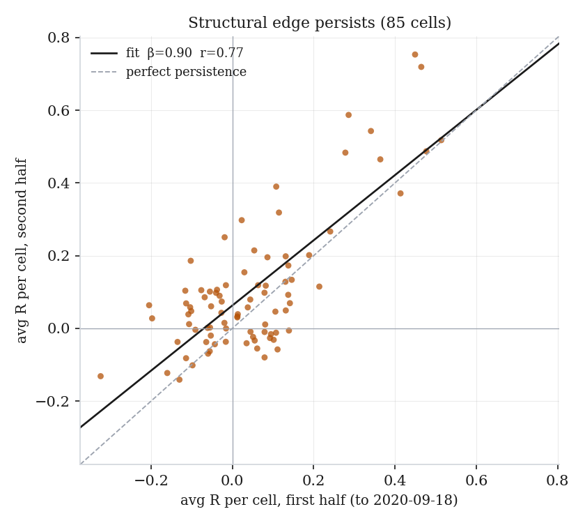
β = 0.90 (SE 0.082, t = 10.9), r = 0.77, 85 cells. A slope of 0.90 means a cell that outperformed by 0.10 R in the first half outperformed by roughly 0.09 R in the second — across a gap of nearly five years.
| First half (to 18 Sep 2020) | → | Second half |
|---|---|---|
| Top quintile +0.288 | → | +0.344 |
| All cells +0.046 | → | +0.110 |
| Bottom quintile −0.129 | → | +0.003 |
The top quintile stays on top. The bottom quintile does not stay at the bottom — it reverts to roughly zero, which is itself informative: persistently bad cells are rarer than persistently good ones.
5. The age of the information barely matters
If an edge decayed over time, recent data would predict better than old data. It does not.
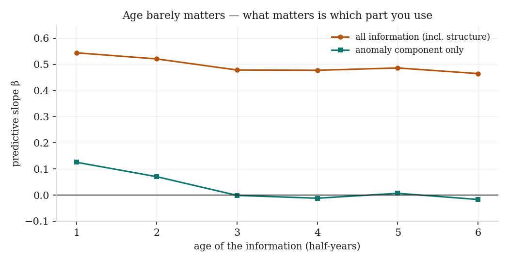
| Age (half-years) | 1 | 2 | 3 | 4 | 5 | 6 |
|---|---|---|---|---|---|---|
| all information | 0.544 | 0.521 | 0.479 | 0.478 | 0.486 | 0.465 |
| anomaly component only | 0.126 | 0.070 | −0.001 | −0.012 | +0.007 | −0.017 |
A half-year from three years ago predicts the next period almost as well (0.465) as the one that just ended (0.544). The information content is essentially flat in age — because it is carried by the structural component, which does not care how old it is.
The gap between the two rows is the honest measure of recency's worth: 0.544 − 0.465 ≈ 0.08. That is what "what just happened" adds over "what has always been true."
The anomaly component is not zero at lag 1 (+0.126). Tested against a permutation null — periods shuffled within each cell, 500 runs — it clears at z = 6.6. So there is a real, tiny momentum in fresh anomalies. It is statistically solid and practically almost irrelevant, and it is gone by lag 3.
6. Two checks that killed our own hypotheses
Regime momentum does not survive detrending. Good half-years do appear to follow good half-years: AR(1) on the regime factor gives β = +0.71 (t = 3.9). But the regime factor also has a mild upward trend across the sample, and a trend alone produces positive autocorrelation. Detrended, it collapses to β = +0.29 (t = 1.4) — not significant. What looked like "momentum in market conditions" was mostly a trend artefact.
Edges do not erode. The obvious worry: as markets get more efficient, the spread between good and bad cells should shrink.
| Epoch | avg R | SD real (spread between cells) |
|---|---|---|
| 2015–2018 | +0.024 | 0.145 |
| 2019–2022 | +0.100 | 0.189 |
| 2023–2026 | +0.115 | 0.164 |
No erosion over 11 years — if anything the opposite. Caveat, and an important one: our setup family was developed with knowledge of recent years, so the later epochs are partly in-sample. The honest reading is "no evidence of erosion", not "proof of none."
What this study cost us. The analysis produced a side effect we did not go looking for: an apparent "similar-days" effect of +0.73 R that was too good. It turned out to be a look-ahead leak — two context features (opening-range levels and a cash-open-derived bias) were being read before they could be known, in 48.8% of episodes. After the fix the effect fell to +0.19 R. The diagnostic that exposed it: the prediction under-stated the outcome, and a noisy predictor must always over-state. All R values in this paper are unaffected — the bug touched features, never results, and every anchor reproduced bit-for-bit after the rebuild. We mention it because a paper on measurement error that hid its own would be worth little.
7. What follows for practice
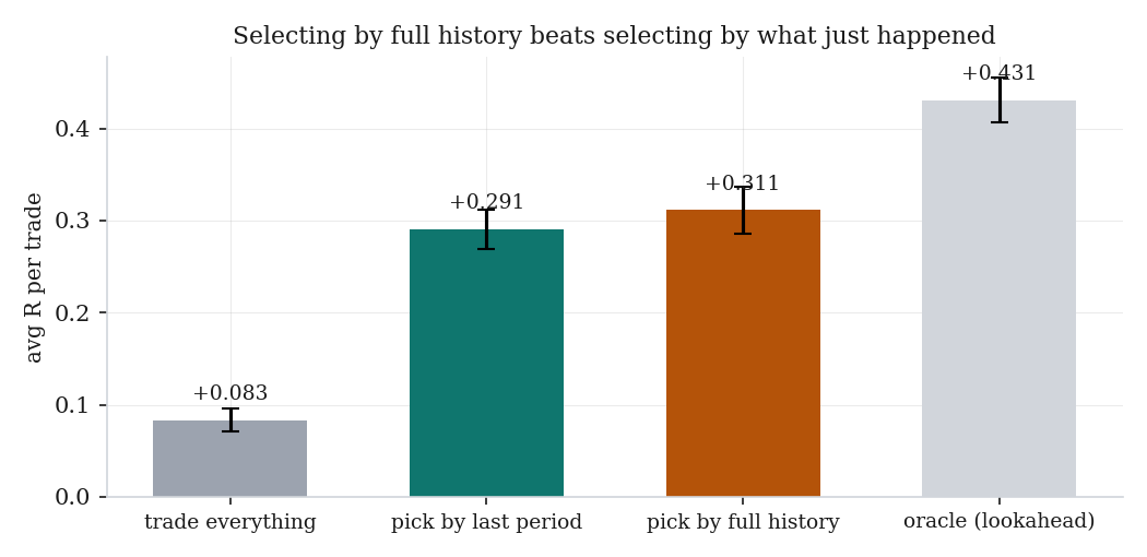
Four selection rules, walk-forward: at each period, cells are picked using only data available before it, then held for that period.
| Rule | avg R per trade |
|---|---|
| Trade everything | +0.083 |
| Pick top quintile by last period | +0.291 |
| Pick top quintile by full history | +0.311 |
| Oracle (perfect foresight) | +0.431 |
Two things stand out. First, selecting by recency works surprisingly well (+0.291) — but not because recency is informative. It works because last period's number is a noisy proxy for the structural edge. Using the full history directly does the same job better.
Second, the gap between the best usable rule (+0.311) and perfect foresight (+0.431) is only 0.12 R. That is the entire space in which any adaptive, timing-based intelligence can operate — and we now know most of what lives in that space is noise.
In a joint regression both components survive: structure β = 0.63 (t = 17.6), recency β = 0.27 (t = 10.8). Recency is not worthless. It is worth roughly a quarter of what structure is worth, and should be weighted accordingly rather than driving the decision.
The practical rule: shrink a fresh reading by about 90% before believing it. Shrink a structural edge by about 10%. The two numbers differ by an order of magnitude, and treating them alike is the most expensive mistake in this data.
8. Limits
- The cell universe is our own setup family — 23 setups selected over years because they looked plausible. The persistence findings are internal comparisons and largely unaffected, but absolute levels are optimistic. This is not a statement about all conceivable patterns.
- One dataset. Every out-of-sample block here comes from the same 11.4 years. As in every study we publish: live forward is the only true out-of-sample.
- Half-years are a choice. Annual buckets give the same picture (structural signal 95%, anomaly 26%), but the exact decay shape depends on bucket length.
- R is fat-tailed. Cell-period means with fewer than 25 trades were excluded; results with n near that bound remain noisy.
- Not tested: whether anomalies behave differently in specific regimes (high volatility, event days). The decomposition treats all periods alike.
The one-sentence version
A structural edge survives five years. A fresh anomaly does not survive six months. Both look identical on the screen — the observed spread differs by less than 10%. Telling them apart is not a matter of experience or instinct. It requires the arithmetic.
📄 Full study as PDF: 9 pages incl. all tables, figures and limits (in German).
Disclaimer: Historical statistics are no guarantee of future market behaviour. This study is not investment advice. Trading involves risk of loss up to total loss.