Data basis: DAX, Dow, Nasdaq CFD M1 data, 24-hour sessions, Jan 2015 to Jun 2026. Percent-reversal ZigZag at four scales: M5 with 0.3% legs (intraday), H1 with 0.6%, 1.0% and 2.0% legs (days to weeks). Pattern A→B→C: swing A, swing B, retracement C that does not exceed A, both directions. 501 to 20,027 patterns per cell. Benchmark: a synthetic market from the same bars, shuffled within calendar month and time-of-day slot, three seeds, identical code. Volatility regime and intraday profile survive the shuffle; every level, leg and trend memory is destroyed. Only the difference real minus synthetic is a measurement. No costs, no trades: this is a question about structure. No trading recommendation.
"Price falls 900 points, bounces 300, and then falls another 900." The measured move is one of the oldest ideas in chart reading: the second leg in the trend direction repeats the first, so the target is known the moment the retracement ends. AB=CD, 1:1 projection, "the second leg equals the first". It feels right because it is often visible after the fact.
We tested it two ways. First as a distribution: how often is the second leg actually the length of the first? Second as a trade: once the retracement C is confirmed, how often does price reach the 1.0 projection before it retakes C, and does anything happen at that level? Both against a synthetic market in which, by construction, nothing is measured.
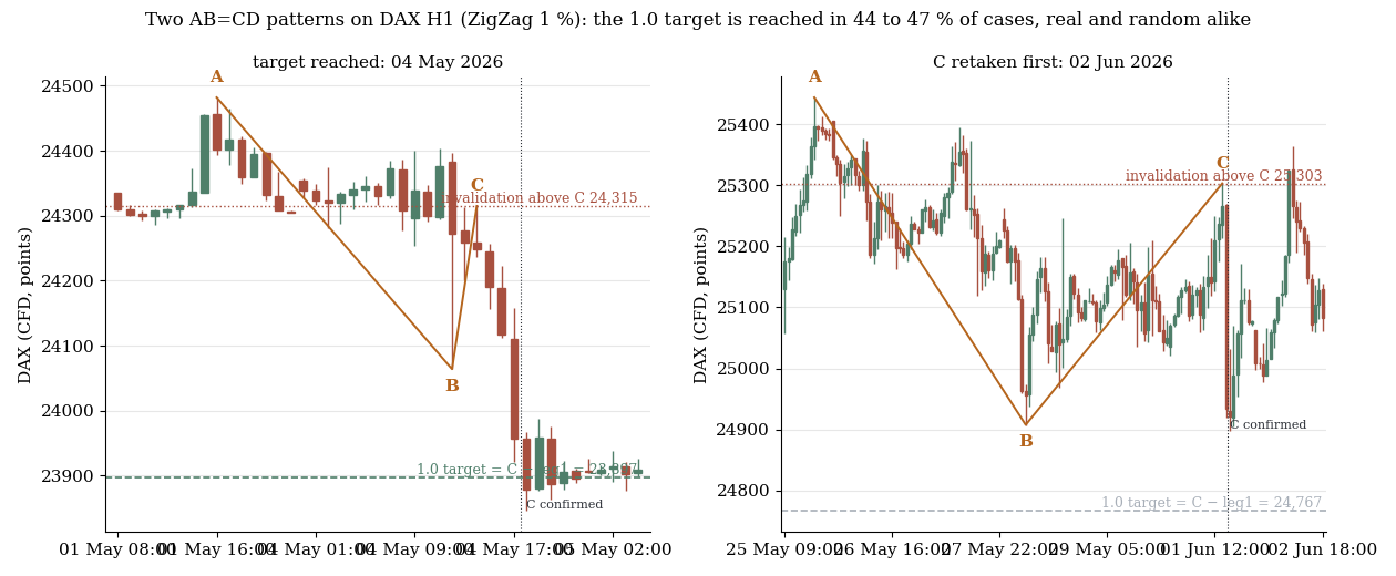
Two patterns on DAX hourly bars with a 1% ZigZag. Left: the projection is reached. Right: price retakes C first. The dotted vertical line marks the bar on which C became known; everything before it is hindsight.
1. The distribution: how long is the second leg?
If the measured move were structure, the ratio of the third leg to the first would cluster near 1. It does not, and it does not in the random market either.
| Cell | n real | Share of leg3/leg1 in [0.9, 1.1): real | synthetic | Δ (pp) | t |
|---|---|---|---|---|---|
| DAX M5 0.3% | 17,679 | 11.8% | 11.7% | +0.1 | +0.3 |
| DAX H1 0.6% | 3,730 | 11.5% | 11.6% | −0.1 | −0.2 |
| DAX H1 1.0% | 1,666 | 10.4% | 11.2% | −0.7 | −0.8 |
| DAX H1 2.0% | 501 | 10.4% | 13.3% | −2.9 | −1.8 |
| DOW M5 0.3% | 12,751 | 11.3% | 11.7% | −0.4 | −1.2 |
| DOW H1 0.6% | 2,693 | 11.4% | 10.8% | +0.6 | +0.9 |
| DOW H1 1.0% | 1,226 | 11.7% | 12.0% | −0.2 | −0.2 |
| DOW H1 2.0% | 386 | 10.1% | 11.8% | −1.7 | −0.9 |
| NQ M5 0.3% | 20,027 | 11.7% | 11.7% | +0.0 | +0.1 |
| NQ H1 0.6% | 4,030 | 11.3% | 10.8% | +0.5 | +0.8 |
| NQ H1 1.0% | 1,960 | 11.5% | 10.3% | +1.2 | +1.4 |
| NQ H1 2.0% | 605 | 13.1% | 10.5% | +2.5 | +1.6 |
One pattern in nine lands within 10% of the 1:1 measure, in the real market and in the shuffled one. The median ratio is 0.75 to 0.79 in every cell, real and synthetic: the typical second leg is three quarters of the first, because a percent ZigZag produces that geometry on any path. Twelve cells, none at |t| ≥ 2.
The "echo" variant, third leg equals the retracement (a double bottom at B), is the one place where the real market differs, and it differs the wrong way: on M5 the exact echo is rarer than random on all three indices (NQ 6.3% vs 7.8%, t = −7.7; DAX 7.2% vs 8.0%, t = −3.5; Dow 7.0% vs 7.9%, t = −3.2). B is either broken or the move turns before it. On H1 the difference disappears.
2. The trade: does price reach the 1.0 target?
The tradeable version starts on the bar on which C is confirmed. From there we ask whether price reaches the projected level C ± k·leg1 before it retakes C, for k = 0.618, 0.8, 1.0, 1.272 and 1.618.
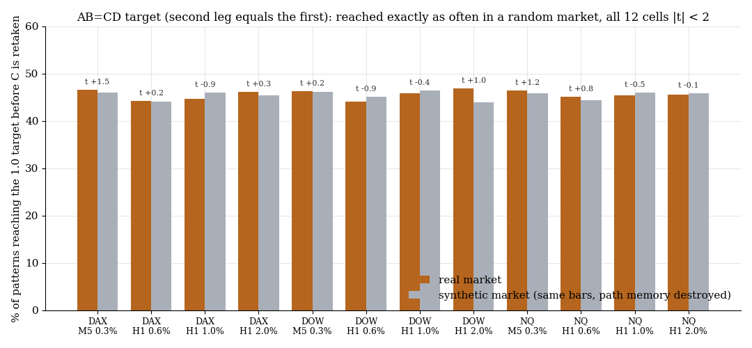
Probability of reaching the 1.0 projection before C is retaken, real versus synthetic, all twelve cells. The t-value above each pair is the difference.
| Cell | P(1.0 reached) real | synthetic | t |
|---|---|---|---|
| DAX M5 0.3% | 46.6% | 45.9% | +1.5 |
| DAX H1 0.6% | 44.3% | 44.1% | +0.2 |
| DAX H1 1.0% | 44.7% | 46.0% | −0.9 |
| DAX H1 2.0% | 46.1% | 45.4% | +0.3 |
| DOW M5 0.3% | 46.2% | 46.1% | +0.2 |
| DOW H1 0.6% | 44.2% | 45.1% | −0.9 |
| DOW H1 1.0% | 45.8% | 46.4% | −0.4 |
| DOW H1 2.0% | 46.9% | 44.0% | +1.0 |
| NQ M5 0.3% | 46.4% | 45.9% | +1.2 |
| NQ H1 0.6% | 45.1% | 44.4% | +0.8 |
| NQ H1 1.0% | 45.4% | 46.0% | −0.5 |
| NQ H1 2.0% | 45.6% | 45.8% | −0.1 |
The 1.0 projection is reached before invalidation in 44 to 47% of real patterns and in 44 to 46% of synthetic ones. Twelve cells, largest |t| 1.5. The same holds for the other four levels: 0.618 is reached about two thirds of the time, 1.618 in 25 to 30% of cases, and the random market gives the same ladder. The numbers are what a percent ZigZag on a volatility-clustered random walk produces; the market adds nothing.
3. Does anything happen at the level?
If 1.0 were a level rather than a number, price should react there: bounce more often at 1.0 than at 0.8 or 1.272, and more often than in the random market. We measure a race after the touch, +0.25·leg1 back against −0.25·leg1 through.
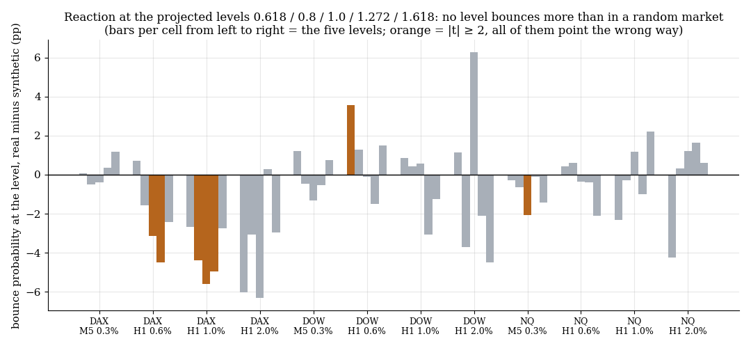
Bounce probability at 0.618, 0.8, 1.0, 1.272 and 1.618, real minus synthetic in percentage points. Orange bars are |t| ≥ 2; every one of them is negative.
At 1.0 the bounce rate is 42 to 51% real against 44 to 50% synthetic. Three cells are significant, all in the same direction: DAX H1 1.0% at −5.6 pp (t = −2.7), DAX H1 0.6% at −3.1 pp (t = −2.2), NQ M5 at −2.1 pp (t = −3.5). Where the real market differs, price runs through the projected level more readily than random, not less. The level contrast, bounce at 1.0 minus the mean of its neighbours 0.8 and 1.272, sits between −4.9 and +1.9 pp in eleven cells; the twelfth, Dow H1 2.0% at +9.2 pp, has 180 patterns and t = 1.4.
4. Why it feels real
The measured move survives because the eye is generous. Given the usual ratio set, 0.5, 0.618, 0.786, 1, 1.272, 1.618 and 2, applied to either the first leg or the retracement, some ratio fits most completed patterns, and it fits them in the random market as well. A trader looking at a chart after the fact will almost always find a measure that "worked", because seven candidate ratios against two candidate legs is fourteen chances per pattern. The projection that looks confirmed in hindsight was one of fourteen, chosen after the outcome.
The forward-looking version of the same idea, pick 1.0 at the moment C is confirmed and hold, is a coin flip with a 45% hit rate, and it is the same coin flip in a market that has no memory.
5. What this means
The measured move is a description of what ZigZag geometry looks like, not a forecast. The second leg is typically three quarters of the first, in real and random data; the 1:1 target is reached in 45% of cases either way; and the level itself provokes no reaction, if anything slightly less than random. This agrees with the Fibonacci study, where the 1.618 extension was reached in 67% of sequences against 71% for a driftless random walk, and with the take-profit study, where a fixed target at a visible level lost against a trailing stop on identical trades.
For a trader the consequence is narrow and practical: do not use a projected 1.0 as a take-profit or as an entry reason. If a trade is open and running, the level is a number on the chart, not a wall.
6. Limits
- The ZigZag threshold is a choice. Four scales cover intraday to multi-week swings; a discretionary reader may define legs differently. We tested the mechanical definition.
- Patterns overlap. A→B→C and B→C→D share legs, so the standard errors are slightly understated. At |t| ≤ 1.6 in every reach cell that does not change the reading.
- The shuffle keeps monthly volatility, not everything below it. A real advantage could also be "volatility persists" rather than "the level works". None appeared, so the caveat cuts the other way: even with that help, nothing.
- No costs, no exits. This is a structure question. A strategy built on the level would carry spread and slippage on top of a 45% coin flip.
- Three indices, one instrument type. FX, single stocks and crypto were not tested.
📄 Full study as PDF: 8 pages incl. all tables, figures and limits (in German).
Disclaimer: Historical statistics are no guarantee of future market behaviour. This study is not investment advice. Trading involves risk of loss up to total loss.