Data basis: DAX, NQ and SPX, M1 data, cash session only, 2015 – 2026. About 35,000 trades per market: one trade every 30 minutes with the direction decided by a coin flip (fixed seed), fixed stop and fixed target in points, exit at the stop, the target or the session end. Costs: today's spread plus slippage assumption (DAX 2.5, NQ 2.5, SPX 0.8 points). The formula is textbook (gambler's ruin); the test checks whether it holds on real prices. No trading recommendation.
This article is deliberately written in plain language. The formula in it is more than 300 years old and reasonably well known in trading blogs as "break-even win rate = 1 / (1 + reward-to-risk ratio)". Still it is missing from almost every strategy pitch that advertises a hit rate. What is new here is not the formula but the test on real prices, the trap in section 5 and the tool that holds your own history against it. There are enough papers nobody reads. Here the explanation comes first, the data second, and the two agree.
1. The drunkard between two ditches
A drunkard stands on a path. One metre to his left there is a ditch. Two metres to his right, a second one. He takes steps, each one randomly left or right, with no preference whatsoever. How often does he fall into the right ditch?
Not half the time. The right ditch is twice as far away, so he has to accumulate twice the distance in one direction. The result is one of the oldest formulas in probability:
P(right ditch first) = distance left / (distance left + distance right) = 1 / (1 + 2) = 33%.
The left ditch is your stop, the right one your target. The drunkard knows nothing about the market. He still reaches the target one time in three. That is the yardstick: the hit rate without any information.
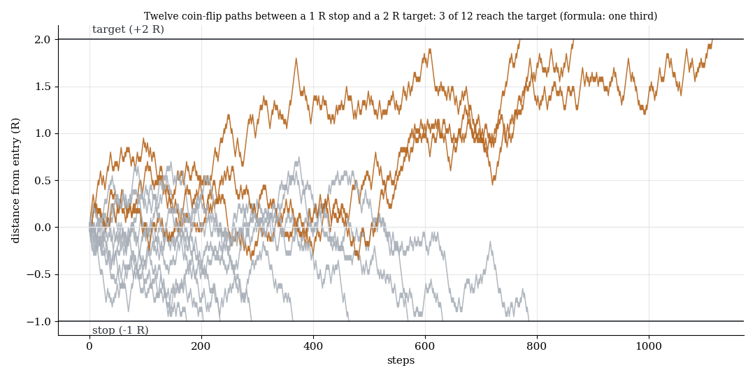
Twelve simulated random paths between a stop at −1 R and a target at +2 R. Orange paths reach the target, grey ones the stop. The formula says one third.
Why exactly this formula? A random walk is fair: on average it stays where it is. If it ends either at −1 (stop) or at +2 (target) and the average has to be zero, then p times (+2) plus (1 − p) times (−1) = 0, so p = 1/3. The formula is nothing but the fairness of chance, solved for p.
2. Why a hit rate alone says nothing
Someone shows you a strategy with a "67% hit rate". Sounds good. But what are its stop and its target? If the stop is twice as far away as the target, the formula says 2 / (2 + 1) = 67% with no edge at all. The drunkard manages that too. The strategy has shown nothing.
The other way round: a strategy with stop 1 and target 5 and a hit rate of 25% sounds weak. The yardstick says 1/6 = 16.7%. So 25% is well above chance. That would be interesting.
A hit rate is never a number you may read on its own. It is always "hit rate minus what chance produces at this stop-to-target ratio". And because every trade has its own ratio, you have to compute it trade by trade.
| Stop : target | chance reaches the target in |
|---|---|
| 1 : 1 | 50.0% |
| 1 : 2 | 33.3% |
| 1 : 5 | 16.7% |
| 1 : 10 | 9.1% |
| 2 : 1 | 66.7% |
| 3 : 1 | 75.0% |
3. The expectation is the honest number, and for chance it is exactly zero
Let us compute the drunkard in R, multiples of the stop. Target = +2 R, stop = −1 R, hit rate 1/3:
Expectation = 1/3 times (+2) plus 2/3 times (−1) = 0.667 − 0.667 = 0.
This holds for every ratio. 1:1, 1:10, 5:1, no matter: for chance the gross expectation is always zero. Tightening the stop or moving the target changes the hit rate, never the expectation. You can push the hit rate wherever you want it. The expectation stays put.
The only number chance leaves behind is the cost. Spread and slippage are paid on every trade; expressed in R:
Net expectation = − cost / stop distance.
A tight stop means the cost eats a larger share. That is why the 2-minute brackets died in our doji study: 2.5 points of cost on an 8-point stop is −0.3 R per trade before anything happens in the market.
From this follows the only clean reading for any strategy: edge = actual average R minus (− cost / stop). If that difference is positive and backed by a t-statistic of at least 2, there is something. A high hit rate alone only says: the stop is wide.
4. The formula on real prices
We let exactly this drunkard loose on real data. DAX, NQ and SPX, eleven years, one trade every 30 minutes with a coin-flip direction, fixed stop, fixed target, evaluated on one-minute candles. About 35,000 trades per market and ratio.
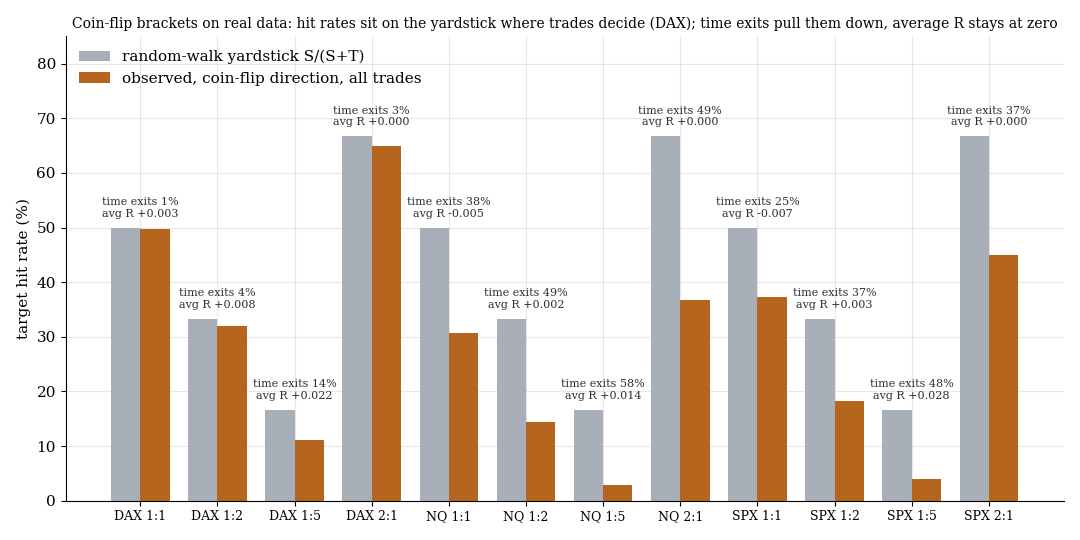
Grey: the formula. Orange: measured. Where the session is long enough for the trade to decide (DAX), the two sit on top of each other. On NQ and SPX the stops are large relative to the movement, many trades end undecided at the session close, and the raw hit rate falls below the yardstick. The average R still stays at zero everywhere.
| Market | Stop : target (points) | n | target hit | yardstick | time exits | avg R gross | avg R net | yardstick net |
|---|---|---|---|---|---|---|---|---|
| DAX | 20 : 20 | 35,196 | 49.8% | 50.0% | 0.8% | +0.003 | −0.122 | −0.125 |
| DAX | 20 : 40 | 35,196 | 31.9% | 33.3% | 3.5% | +0.008 | −0.117 | −0.125 |
| DAX | 20 : 100 | 35,196 | 11.2% | 16.7% | 13.7% | +0.022 | −0.103 | −0.125 |
| DAX | 40 : 20 | 35,196 | 65.0% | 66.7% | 3.4% | 0.000 | −0.062 | −0.062 |
| NQ | 40 : 40 | 34,755 | 30.7% | 50.0% | 38.1% | −0.005 | −0.068 | −0.062 |
| NQ | 40 : 80 | 34,755 | 14.5% | 33.3% | 48.6% | +0.002 | −0.060 | −0.062 |
| NQ | 40 : 200 | 34,755 | 2.8% | 16.7% | 57.8% | +0.014 | −0.049 | −0.062 |
| NQ | 80 : 40 | 34,755 | 36.8% | 66.7% | 48.7% | 0.000 | −0.031 | −0.031 |
| SPX | 8 : 8 | 34,734 | 37.2% | 50.0% | 24.9% | −0.007 | −0.107 | −0.100 |
| SPX | 8 : 16 | 34,734 | 18.2% | 33.3% | 36.8% | +0.003 | −0.097 | −0.100 |
| SPX | 8 : 40 | 34,734 | 4.0% | 16.7% | 47.9% | +0.028 | −0.072 | −0.100 |
| SPX | 16 : 8 | 34,734 | 45.0% | 66.7% | 37.0% | 0.000 | −0.050 | −0.050 |
Three things are in this table. First: on the DAX the formula is right within one or two percentage points at 1:1, 1:2 and 2:1, where almost every trade still decides within the session; at 1:5 it misses by 5.5 points because 14% of the trades are undecided at the session end. The gross expectations sit between −0.007 and +0.028 R. With standard errors clustered by trading day, eleven of the twelve cells stay below |t| = 2, the SPX 1:5 cell sits at 2.9, and all three 1:5 cells are positive. A different coin-flip sequence moves these wide brackets by about one standard error; the effective sample is much smaller than the trade count suggests. We read the table as consistent with zero, with the wide targets as an open question rather than a finding. Second: the net column is nothing but cost divided by stop, exactly as predicted. Third: on NQ and SPX the raw hit rate falls far below the yardstick because many trades end undecided. The expectation does not. Which leads to the most important section.
5. The trap: "we only count completed trades"
Some trades reach neither stop nor target by the session end. What to do? The common answer: "We don't count those, we only count the decided ones." Sounds clean. It is not.
Numbers from the NQ, stop 40 and target 200, a 1:5 bracket. The yardstick says 16.7%. Decided trades only: 6.6%, with a z-score of −33. That looks like a massive anti-edge. It is not one. The target is five times as far away as the stop and therefore needs much more time. The trades that are decided by the session end are disproportionately the ones that hit the near stop. The sample was distorted by the rule, not by the market.
With the reversed ratio (stop 80, target 40) the opposite happens: 71.7% instead of 66.7%. Now the target is the near barrier, and "decided" favours it. That looks like an edge and is again just selection.
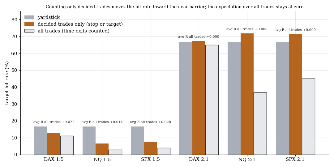
Orange: decided trades only. At 1:5 the hit rate falls below the yardstick, at 2:1 it rises above it. Both without anything happening in the market. The expectation over all trades, with time exits valued at the closing price, is zero in every cell.
| Market | Stop : target | decided only, n | target hit | yardstick | z | avg R, all trades |
|---|---|---|---|---|---|---|
| DAX | 20 : 100 | 30,371 | 13.0% | 16.7% | −17.4 | +0.022 |
| NQ | 40 : 200 | 14,657 | 6.6% | 16.7% | −32.7 | +0.014 |
| SPX | 8 : 40 | 18,112 | 7.7% | 16.7% | −32.4 | +0.028 |
| DAX | 40 : 20 | 33,994 | 67.3% | 66.7% | +2.3 | 0.000 |
| NQ | 80 : 40 | 17,827 | 71.7% | 66.7% | +14.4 | 0.000 |
| SPX | 16 : 8 | 21,899 | 71.3% | 66.7% | +14.6 | 0.000 |
Hit rates depend on your time limit. Expectations do not. Whoever counts only completed trades measures their holding time, not their strategy.
6. Three claims against the yardstick
The yardstick is a tool, not a result. Three examples from our own tests, all with the same logic:
"Every 50% Fibonacci retracement gets sold." Rephrased: how often is the low broken before the high is reclaimed? The drunkard says: distance to the high divided by (distance high plus distance low). Measured across DAX, Dow and NQ in 36 cells by retracement depth: deviations between −10 and +11 percentage points, with alternating sign. The Fibonacci level is geometry, not a signal.
Opening-range breakout with a 10 R target. A well-known study trades the direction of the first 5-minute candle with the stop at the candle's extreme and the target at 10 R. The yardstick says 1/11 = 9.1% target hits. Measured on index CFDs over eleven years: 2.6 to 4.2%, less than chance, because the session is too short for a 10 R target (section 5). The "24% hit rate" quoted in the study is the win rate including closing-price exits, a different number. The gross expectation of +0.13 R is real; the costs are −0.22 R. One sentence with the yardstick says both.
Targets at "important levels". A target at the previous day's high instead of at 2 R changes the distance and with it the hit rate, exactly as the formula predicts. It does not change the expectation. That is why, in our tests, every fixed level target lost against a trailing exit: the level moves the hit rate, but the system lives on the right tail of the distribution, which a fixed target cuts off.
7. And if the market has a drift?
The drunkard has no preference. Indices, however, rise in the long run. So a long trade should reach the target more often than the formula says. The question is by how much, and how to measure it.
The formula with drift. A random walk with drift μ (mean move per minute) and volatility σ (standard deviation per minute) has a single number that matters: θ = 2μ / σ². With it the simple formula becomes
P(target first) = (1 − e^(−θ·S)) / (1 − e^(−θ·(S+T)))
with S and T as distances in percent of price. As θ goes to zero, S / (S+T) comes back. A short trade sees the same formula with −θ. This is the complete version of the yardstick; the formula in section 1 is its special case without drift.
Measuring the drift. Take the intraday return of every day, from the opening price of the first session minute to the closing price of the last, without the overnight jump, and average. The definition is not a detail: using the close of the first minute instead of its open changes the DAX drift from −0.1 to +0.5 basis points, because the first minute of trading runs up on average. Add the standard error, otherwise you believe numbers that are not there. Eleven years, about 2,900 days per market:
| Market | intraday drift per day | standard error | t | annualised | σ per day | θ |
|---|---|---|---|---|---|---|
| DAX | −0.1 basis points | 1.7 bp | −0.1 | −0.3% | 0.93% | −0.3 |
| NQ | +3.6 bp | 2.0 bp | 1.8 | +9.0% | 1.04% | +6.6 |
| SPX | +2.3 bp | 1.5 bp | 1.5 | +5.9% | 0.84% | +6.6 |
This is the honest core: after eleven years the intraday drift is statistically indistinguishable from zero. Even on the NQ it sits at 1.8 standard errors, just below the usual threshold of 2. The standard error of a drift shrinks only with the square root of the years; to establish +3.6 basis points with t = 2 safely you would need about 14 years, on the SPX about 20. The long-run rise of the indices is real, but it happens overnight, not in the session an intraday bracket lives in.
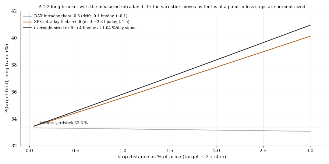
A 1:2 long bracket with the measured intraday drift: the yardstick moves by tenths of a point as long as the stop is small against the price. Only with percent-sized stops, i.e. trades held over days, does the drift become visible.
What the drift changes on the yardstick. For the brackets in section 4 it moves the hit rate by less than 0.1 to 1.2 percentage points and the expectation by 0.001 to 0.035 R. We checked it, this time not with a coin flip but with every trade once long and once short:
| Market | stop : target | long avg R | short avg R | drift formula expects long / short | standard error |
|---|---|---|---|---|---|
| DAX | 20 : 40 | +0.020 | −0.011 | +0.001 / −0.001 | 0.007 |
| NQ | 40 : 80 | +0.029 | −0.021 | +0.035 / −0.035 | 0.006 |
| SPX | 8 : 16 | +0.025 | −0.020 | +0.019 / −0.019 | 0.006 |
On NQ and SPX the drift formula matches the measured long-short asymmetry in magnitude. On the DAX the measured asymmetry is larger than the practically absent drift explains; that stays on record as an open point and is a candidate for a test of its own. In all cases the effect is two to three hundredths of an R per trade, against costs of 0.06 to 0.12 R. The drift is real, small, and it does not pay the spread.
How to integrate it. First measure the drift on the time scale of the trade (intraday trades: intraday drift; swing trades held overnight: drift including the overnight part), then look at the standard error, then compute θ and use the formula with drift as the yardstick. Whoever derives θ from a drift without a standard error builds an edge out of noise. The MQL5 script in the companion material computes both and prints the standard error alongside.
8. Where the yardstick does not hold
Gaps. A gap jumps over the ditch. Then the loss is larger than 1 R. The formula assumes the path touches every point.
Coarse evaluation. If you simulate on candles almost as large as the stop, you do not know which barrier was touched first, and you tend to credit the trade with the overshoot. In our doji study exactly that produced +0.16 R out of nothing. That is an article of its own.
9. What to do with it
Before every optimisation, one question: what would my hit rate be if I knew nothing? The answer is in section 1, with drift in section 7. Then two numbers instead of one: target hits against the yardstick with a z-score, and average R against −cost/stop with a t-statistic. If only the hit rate is high, you have a wide stop. If the R is above the yardstick and the t-statistic above 2, you have something worth investigating further.
The yardstick does not find edges. It removes the illusion of one.
Caveat: The coin-flip trades are not a trading system and are not optimised. Costs are today's spread assumptions applied to old prices; the early years are therefore priced rather too expensively. Candles touching both barriers were counted as a stop (conservative). All numbers come from a chain that first reproduced a known value (the overnight/intraday decomposition).
📄 Full study as PDF: 10 pages incl. all tables, figures and limits (in German).
Disclaimer: Historical statistics are no guarantee of future market behaviour. This study is not investment advice. Trading involves risk of loss up to total loss.